Notes on The Little Learner

The Little Learner is a book in the Little book series written by Dan Friedman and several coauthors. The aim of the book is to provide a solid understanding of the computational ideas behind Deep Learning using Scheme as the programming language.

⊕The end game of at least one of the authors of the book is to use Scheme’s rich compiler ecosystem to generate efficient code for FPGAs and/or GPUs, under the belief that Lisp compiler techniques will yield better results than the current approach. While Scheme is not widely used in this domain, it is an excellent choice for this hands-on book because the authors need use only a very small subset of an already compact language, thus requiring little ramp up from the reader. Additionally, since functions are first-class values in Scheme, we can pass them as arguments to functions, and functions can also return functions. This will result in extremely clear and compact code that can be understood easily.

The book uses a unique format of question and response: each page is divided into frames, where the left side of the frame poses a question or idea, and the right side provides an answer or hint for how to proceed. The learning process entails reading the prompt, mulling it over, perhaps proposing a solution, and then checking the right side of the frame. This approach often requires writing a bit of code, with the goal of ensuring that the reader understands all the details fully. But, as noted in other books in the series, while the book provides some distillation of the content in terms of laws and rules, it is up to readers to take notes, write down their own definitions, and ensure that they understand the ideas fully. These notes are my attempt to make sense of the Littler Learner.

The text below is organized according to the book and uses headings from the chapters and interludes as a guide.

The Lines Sleep Tonight

Having functions as first-class values makes it possible to write the general equation for a line:

(define line
  (lambda (x)
    (lambda (w b)
      (+ (* w x) b))))

so invoking (line 4) returns the function

(lambda (w b)
  (+ (* w 4) b))

which corresponds to a parameterization of all lines that have 4 as the $$x$$ coordinate in terms of a slope $$w$$ and intercept $$b$$ . This seems backwards from the usual way we think about lines, but it is the right way to look at lines when our task is to estimate the slope and intercept for a given set $$S$$ of training points.

More formally, for this definition of line, $$x$$ is the formal and $$w$$ and $$b$$ are the parameters, since line is a parameterized function, i.e., a function for that accepts parameters after the formals are known. We aim to established the value of the parameters $$w$$ and $$b$$ given a set of values for $$x$$ along with their corresponding values $$y$$ .

As an example, consider the graph below:

⊕The aim of The Little Learner is to provide readers with the understanding for how to estimate parameters such as w and b so that we can use them to predict y values for arbitrary values of x.

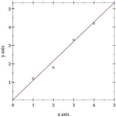
The red line corresponds to the line $$wx + b$$ , where $$w$$ and $$b$$ have been inferred using the techniques of machine learning from a set $$S$$ of points $$(x, y)$$ depicted in the graph. ⊕The other lines would have slightly different parameters $$w$$ and $$b$$ corresponding to various loss functions. More on this below. There are other lines that could have been generated using machine learning techniques. These parameters $$w$$ and $$b$$ are collectively referred to as $\theta$ : $$w$$ is the first element of $\theta$ , which we denote as $\theta_0$ . and $$b$$ is the second element of $\theta$ , which is $\theta_{1}$ .

⊕It turns out that Emacs supports the use of Unicode, so most of my code uses Greek letters, e.g., $\theta$ instead of theta. All the code in the book uses Greek letters but the lookup page tells us to use text instead, e.g., theta. The book uses lists for parameters, hence $\theta_0$ is represented in code with (first theta) and corresponds to $$w$$ . Likewise, $\theta_1$ is represented as (second theta) and corresponds to $$b$$ .

The More We Learn the Tenser We Become

⊕We can think of tensors of rank 1 as vectors and tensors of rank 2 as matrices. For convenience, we treat scalars as tensors of rank 0. Tensors are a data structure that is used to hold data. Generally, a tensor $$t$$ is container with rank $$n$$ which corresponds to the nesting of the elements constituting the vector. More precisely, a tensor $$t$$ of rank $$1$$ is comprised of $$k$$ scalars. We define its length to be $$k$$ , with the corresponding scheme function being tlen. Tensors of rank $$2$$ are constructed from tensors of rank 1, each of which will have the same length $$n$$ . A tensor of rank $$n + 1$$ is constructed from tensors of rank $$n$$ , where, again, each has the same length. Note that the rules for tensor construction require that all the elements of a tensor of rank $$n$$ have the same structure or shape. We write a tensor of rank $$n$$ as $t^{n}$ .

Example of a tensor of rank 1:

(define line-xs
  (tensor 2 1 4 3))

and a tensor of rank 2:

(tensor (tensor 7 6 2 5)
          (tensor 3 8 6 9)
          (tensor 9 4 8 5))

The length of a tensor $$t$$ corresponds to (length t) in Scheme.

⊕Thinking of tensors as trees is a conceptual exercise. Their implementation can vary depending on the circumstances. We can think of tensors as trees: a tensor $$t^k$$ is a tree of depth k, where the nodes in each level of the tree have the same number of branches, and the leaves are scalars. The function tlen gives us the branching factor of the first layer; we can access the ith branch with (tref t n), where t is the tensor, and n is the nth branch in the tree.

We mentioned shape above. The shape of a tensor $$t^m$$ is a list where the first number is the number of elements of $$t$$ , the second is the number of elements in $$t_0$$ (actually, any of the elements will do as well), the third number will the the number of elements one level down, i.e., (tref (tref t 0) 0), etc. These relationships are codified as

(define shape
  (lambda (t)
    (cond
      ((scalar? t) '())
      (else (cons (tlen t) (shape (tref t 0)))))))

Remarks:

The tensors $$t^m$$ that are the elements of tensor $t^{m+1}$ must all have the same shape. The rank of a tensor t is the length of its shape, i.e., (length (shape t)).

The More We Extend, the Less Tensor We Get

As mentioned above, we can think of tensors as a tree-like data structure but we haven’t discussed their purpose, which relies on the notion of extension. The main idea is that we can extend functions by extending the behaviour of a function from a base case.

Take $$+$$ : we can extend its behaviour to tensors by descending recursively into its arguments until we operate on scalars–made possible by the regular shape of tensors.

(+ (tensor (tensor 4 6 7) (tensor 2 0 1))
   (tensor (tensor 1 2 2) (tensor 6 3 1)))
;; => (tensor (tensor 5 8 9) (tensor 8 3 2))

Note that the structure of the result is the same as the structure of its arguments. We can use $$+$$ with tensors of different shape:

(+ 4 (tensor (tensor (tensor 1 2 3))
             (tensor (tensor 4 5 6))))
;; => (tensor (tensor (tensor 5 6 7)) (tensor (tensor 8 9 10)))

We can think of going inside the tensor for the operation. In the first example, we descend into the tensors until we get down to scalars and then tally those up respecting the structure of the tensors; in the second example, the $$4$$ is added to the inner scalars, again respecting the structure of the tensors.

The way extension works isn’t always obvious:

(+ (tensor 1 2) (tensor (tensor 3 4)
                        (tensor 5 6)))
;; => (tensor (tensor 4 5) (tensor 7 8))

but

(+ (tensor 1 2) (tensor (tensor 3 4)
                        (tensor 5 6)
                        (tensor 7 8)))
;; => (tensor (tensor 4 6) (tensor 6 8) (tensor 8 10))

Extended operations need not have scalars as their base computation. Consider $$sum^1$$ , which operates on tensors of rank 1 by computing the sum of their elements.

We can define $$sum$$ as an extension of $$sum$$ so that

(sum (tensor (tensor (tensor 1 2) (tensor 3 4))
             (tensor (tensor 5 6) (tensor 7 8))))
;;=> (tensor (tensor 3.0 7.0) (tensor 11.0 15.0))

Note that the rank of $$sum$$ operating on a tensor of rank $$m$$ will be a tensor of rank $$m - 1$$ .

The text has a detailed explanation of extensions later on, so we defer the discussion. More importantly, any function defined using extended functions is itself an extended function:

(sqrt 9)
;; => 3

(sqrt (tensor 9 16))
;; (tensor 3 4)

(sqrt (tensor (tensor 4 9 16) (tensor 25 36 49)))
;; => (tensor (tensor 2 3 4) (tensor 5 6 7))

More importantly for us, we can use line on tensors because it is an extended function. Tensors provide a helpful container for computing predicted ys from the tensor of xs, given a list of parameters $\theta$ .

(define line
  (lambda (x)
    (lambda (theta)
      (+ (* (first theta) x) (second theta)))))

((line (tensor 2 7 5 11)) (list 4 6))
;; => (tensor 14 34 26 50)

Running Down a Slippery Slope

The problem: given a parameterized function parm-fn, i.e., a function of the form

(defn parm-fn
  (lambda (x)
    (lambda (theta)
      ...)))

and a set of inputs $$xs$$ , along with their corresponding $$ys$$ , we want to find the value of $\theta$ that provides the best fit, so that applying parm-fs to the $$xs$$ gives us values of $$y$$ that are “close” to the given $$ys$$ .

We need to do a couple of things: first, we need to find estimates for $\theta$ and, second, we need to quantify how good an estimate is. We use a loss function to determine the fit. Recall from a previous section that the predicted values of y can be computed with

((parm-fn xs) theta)

so we can compare the predicted values of y to the given ys by applying the loss function, which for now is defined to be

(define l2-loss
  (lambda (target)
    (lambda (xs ys)
      (lambda (theta)
        (let ((pred-ys ((target xs) theta)))
          (sum (sqr (- ys pred-ys))))))))

⊕The computation in Scheme would have required the use of reduce and map, or an equivalent approach. where target is the parameterized function, e.g,. parm-fn. Note the economy of expression due to the use of tensors.

A bit of terminology: consider the (l2-loss line), where line is the value of target in the definition of l2-loss. This function application returns

(lambda (xs ys)
    (lambda (theta)
      (let ((pred-ys ((line xs) theta)))
        (sum (sqr (- ys pred-ys))))))

which is called the expectant function (because it expects inputs xs and ys). The application of the expectanct function with actual values for its parameters yields the objective function:

(lambda (theta)
  (let ((pred-ys ((line xs) theta)))
     (sum (sqr (- ys pred-ys)))))

Now that we know how to quantify the goodness of fit for $\theta$ , we turn our attention to the business of estimating it. Start with 0 as the value of theta. Figure out the rate of change of the current theta by adding a small number to it, computing the new value of the objective function, and then its rate of change:

$r = \frac{L2_1 - L2_0}{\Delta\theta}$

where $$L2$$ stands for the l2-loss function. $$r$$ quantifies the impact on l2-loss when we change $\theta$ a little. Now, armed with an estimate for the rate of change, we can improve our estimate of $\theta$ by adding or subtracting a small number from it.

Assume that the change in the change in $\theta$ that we used to compute the rate of change of l2-loss is positive. If $$r$$ is positive, this means that we need to subtract a small number from $\theta$ to compute the next $\theta$ –not the number that we used to compute the rate of change, but a judiciously chosen perturbation for the next iteration of $\theta$ . We want to subtract a bigger number when $$r$$ is large and a smaller one when $$r$$ is smaller, but we avoid using $$r$$ because it might be too large. Thus, we subtract a fraction $\alpha$ of the rate of change so

$\theta_1 = \theta_0 - \alpha \times r$

where $$r$$ is the rate of change we computed above.

Conversely, if the rate of change $$r$$ is negative, we then want to increase $\theta_0$ to reduce the loss. Thus, we also subract a fraction $$r$$ of the (negative) rate of change, which results in $\theta_1 > \theta_0$ , so the equation above also holds. $\alpha$ is called the learning rate.

Slip-slidin’ Away

The graph above with four points and a line passing through them depicts the data set that the book has been using, with the line being a visual approximation of a function that might be used to estimate the value of y for an arbitrary x. Do note that the line intersects the origin, or very nearly so. This means that we can descibe the parameter for the line, $\theta$ as $\theta_0 = m$ for some $$m$$ , and $\theta_1 = 0$ .

Since the line we have fitted is a good approximation, we can then plot the l2-loss vs. all the possible values for $\theta_0$ .

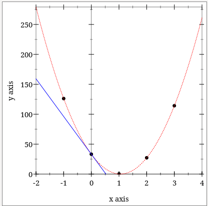
The black points correspond to our data set. Notice that the l2-loss is zero or very close to it for $$x = 1$$ . Note also the line in blue: it is the tangent to the l2-loss function for $$x=0$$ . Much like in the discussion in the previous chapter, the negative slope indicates that an increase in $\theta_0$ will result in a lower value for l2-loss, meaning that the new $\theta_0$ would improve the fit. Note also that the slope of the tangent line decreases as we move away from 0 towards 1.